LCnetgen Example 6, VLF Loop Receiver

This is a large area rectangular loop made from 3-core mains cable, connected to a transimpedance amplifier in order to produce a broadband response.

Input file

Input file loop1.in contains

   
   width = 12  ; 12 metres wide
   height = 2  ; 2 metres high
   base = 0.05 ; base of loop almost at ground level
   
   coil { ; Loop in xz plane (east-west response)
   
      name loop
   
      end1 { -width/2, 0, base }            ; Lower west corner
           { -width/2, 0, base + height}    ; Upper west corner
           {  width/2, 0, base + height}    ; Upper east corner
           {  width/2, 0, base }            ; Lower east corner
   
      length 0
      turns 3
      wirad 0.6e-3
   }
   
   ground { center 0,0,0 axis 0,0 }   ; Horizontal ground at z = 0
   
   field { magnetic 90,90 }   ; Magnetic field in +y direction to
                              ; represent EM wave arriving from east/west

The lower leg of the loop runs along the ground but we cannot set base = 0 in the model because the wire would intersect the ground, so to start with, a base height of 5cm is used.

The command

   lcng -o list loop1 && cat loop1.list

produces something like

   C L1_0 inf 2.47801e-10
   L L1_0 self 3.51760e-04
   L L1 self 3.51760e-04
   R L1_1 1.29977e+00

which shows that the effective inductance of the loop is 352 uH. If the ground statement is commented out and the command re-run, the inductance becomes 399 uH. The inductance of the loop is being significantly affected by the close proximity of a perfect ground. The measured inductance of this loop is 375 uH which shows that the actual ground below the loop is not so perfect.

A few minutes of trial runs with a range of coil base heights determines that a value of 18cm reproduces the measured inductance. Therefore the remainder of this simulation substitutes base = 0.18 in the input file.

lcng is predicting a resistance of 1.3 ohms and the measured value is 1.4 ohms which is close enough considering the accuracy of the ohmmeter.

The next step is to produce a Spice sub-circuit with

   lcng -o spice loop1

and inspecting the file loop1.spice reveals the pin assignments

* pin 1: zero of potential at infinity
* pin 2: LOOP end1, 0.00 turns
* pin 3: LOOP end2, 3.00 turns
* pin 4: B-field, 1 amp = 1 Tesla

which we need to use in a Spice model of the receiver.

Receiver Circuit

A Spice test circuit can easily be constructed by hand for this simple preamp, but this example will demonstrate the use of gEDA. lcng can produce a gEDA symbol for this coil with the command

   lcng -o geda loop1

which produces a gEDA symbol file loop1.sym. Make sure your working directory is included in the symbol search path used by gEDA. If necessary, edit or create ~/.gEDA/gafrc and add your working directory with

(component-library "/your/directory")

Then after restarting gschem you should find loop1.sym in the component library.

Use gschem to draw a schematic and include loop1 as a sub-circuit. It needs two attributes: value=loop1 and file=loop1.spice.

In this example, Ct1-6 and Rt1-2 account for the measured resistances and capacitances of the coupling transformer Lt1-2 and K1 is its measured coupling coefficient. Rd is a dummy high value noiseless resistor necessary so that Spice can determine a DC operating point for that part of the circuit which would otherwise be floating. Vout is a netname attribute assigned to the output net of the LT1028 - this allows the Spice simulation to find the output node. Current source IB is set to 1e-15 to produce a 1 fT field. This is quite a weak flux density but would be considered a fairly strong VLF amateur radio signal.

The schematic is saved as loop1.sch and a Spice netlist generated with the command

   gnetlist -g spice-sdb -o loop1.net loop1.sch

This netlist does not contain any of the Spice commands which tell Spice what to calculate and plot. They could be added to the schematic using the gEDA Spice directive components. More conveniently for this example, the Spice commands are put into a file loop1-test.spice which contains a statement to include loop1.net

File loop1-test.spice contains

   .include loop1.net
   .control
   op
   ac dec 100 10 1000k
   noise V(Vout) IB dec 100 10 1000k
   setplot ac
   wrdata /tmp/t1 V(Vout)
   setplot noise1
   wrdata /tmp/t2 sqrt(onoise_spectrum)
   .endc

Running this with

   ngspice -b loop1-test.spice

produces two data files /tmp/t1.data and /tmp/t2.data and these are plotted below:

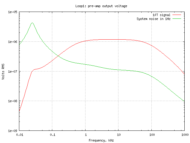
The response is reasonably flat from around 500Hz to 100kHz and the 1 fT signal appears about 20dB above system noise at the 8kHz band used by radio amateurs. The measured system noise at 8kHz corresponds to a flux density of about 0.15 fT which agrees quite well with the model. This is more a matter of luck than judgement - Spice predictions of noise can differ quite a lot from measured noise for various reasons.

Output voltages are very low - this is typical of loop antennas feeding a transimpedance amplifier and at least one or two further gain stages are necessary to produce a line level signal.