LCnetgen Example 1, Tesla Coil

This example models the Tesla coil 'Thor' which was built as a postgrad research project by Marco Denicolai. It is a very well documented and measured system and therefore a good test case for LCnetgen.

Thor website .

Input file

Input file thor.in contains

   electrode {
   
      name ground
   
      disc {    ; Floor
        radius 5
        center 0,0,0
        axis 0,0
      }
   
      cylinder { ; Walls
        radius 5
        end1 0,0,0
        axis 0,0
        length 6
      }
   
      disc {    ; Roof
        radius 5
        center 0,0,6
        axis 0,0
      }
   }
   
   electrode { ; Toroidal topload
   
      name topload
   
      toroid {
         outer_radius 0.7575
         inner_radius 0.5575
         center 0,0,2.85
         axis 0,0
      }
   }
   
   coil {   ; Flat spiral primary
   
      name primary
   
      radius1 0.275
      radius2 0.545
      end1 0,0, 0.995 + 51e-3    ; Set for measured k=0.187
      length 0    ; Flat spiral, therefore zero length
      axis 0,0    ; Vertical axis
      turns 9.5
      tap 7.5
      wirad 0.4e-2
   }
   
   coil  {   ; Cylindrical secondary
   
      name secondary
   
      radius 0.20
      length 1.575
      end1 0,0, 0.995
      axis 0,0     ; Vertical axis
      turns -939
      wirad 0.725e-3
   }

Generate a Spice sub-circuit and a tiles file from thor.in with the command

   lcng -o spice -o tiles thor

View the system (excluding the floor, walls and roof) with the gnuplot commands

   set terminal x11
   set style data dots
   set view equal xyz
   set xrange [-1.5:1.5]
   set yrange [-1.5:1.5]
   set zrange [0.8:3.8]
   set grid
   set xyplane 0
   unset key
   splot 'thor.tiles' using 1:2:3

to get something like

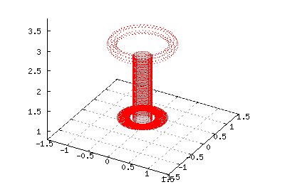
Test Circuit One - Steady State Response

This circuit just injects an AC voltage into the secondary base so that we can see where the resonances are from a plot of the top voltage. The Spice file thor-steady.spice contains

   Thor
   .OPTIONS NOMOD NOPAGE
   .AC LIN 10K 1K 600K
   .PRINT AC V(2)
   
   .INCLUDE thor.spice
   
   * 1 volt AC applied to base
   Vin 0 1 DC 0 AC 1.0
   
   X1 0 2 0 1 2 0 3 4 thor 
   .END

Run the above Spice circuit with something like

   ngspice -b thor-steady.spice > thor-steady.out

Plotting the secondary voltage produces

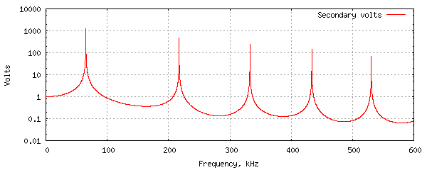
The resonant frequencies taken from the plot can be compared with Marco's measurements of the lowest three resonances of the secondary:

   1/4 wave:   measured =  65.5kHz, modelled =  65.1kHz,  error = -0.6%
   3/4 wave:   measured = 222.8kHz, modelled = 217.25kHz, error = -2.5%
   5/4 wave:   measured = 346.3kHz, modelled = 332.9kHz,  error = -3.9%

Test Circuit Two - Transient Response

Thor is fired with the 96.7nF primary capacitor charged to 14kV. The Spice file thor-trans.spice contains

   Thor
   .OPTIONS NOMOD NOPAGE
   
   .TRAN 100nS 400uS UIC
   .PRINT TRAN I(VP) I(VB) V(10)
   
   .INCLUDE thor.spice
   
   VP 0 1 DC 0 AC 0
   RGAP 1 2 1.0
   CPRI 2 3 96.7n  ic=14KV
   
   VB 0 6 DC 0 AC 0
   X1 0 10 0 6 10 0 3 5 thor
   RL 10 0 50000K
   
   .END

Run this with the command

   ngspice -b thor-trans.spice > thor-trans.out

With Tesla coils, the secondary base current waveform provides the best diagnostic. The following graph compares the modelled base current with the actual base current waveform recorded by Marco.